RR Lyrae in the inner Galaxy

At the last group meeting we discussed several issues revolving around RRL in the galaxy. a) Maddie Lucey's paper: she did the selection function using the Rybizki and Drimmel trick. Do we have to do it a la Cantat-Gauding, with the VIVACE and DES as the 'ground-truth' sample b) the poor old heart and RRL. The Vivace sample shows a tight know of RRL at the very center. The distance modulus spread (after extinction correction) is only sigma = 0.25mag. Or 12% of 1.0 kpc at 8.1 kpc. Plan: do light-curved based metallicities and get the spatial structure...

Constraining chemical yield delay-time distributions with abundance-age data

Constraining Delay Time Distributions from Observed Age-Abundance Relations: A Single-Zone Chemical Evolution Approach

Abstract

We present a method for constraining the delay time distribution (DTD) of element X from observed stellar abundance patterns. Using the single-zone chemical evolution framework of Weinberg et al. (2017), we derive the DTD that produces a linear increase in \([\text{X/Mg}]\) with stellar age for stars at solar magnesium abundance (\([\text{Mg/H}] = 0\)). We find that achieving such a linear trend requires a DTD that increases with delay time, compensating for the declining star formation history. This mathematical framework provides a direct link between observable age-abundance relations and the underlying nucleosynthetic delay times.

1. Introduction

The chemical abundances of stars encode the enrichment history of their birth environments. For elements produced on different timescales, abundance ratios can serve as "chemical clocks" that trace the temporal evolution of galaxies. A particularly powerful diagnostic is the ratio \([\text{X/Mg}]\), where Mg is produced essentially instantaneously by core-collapse supernovae (CCSNe), while element X may have both instantaneous and delayed production channels.

The key question we address is: Can chemical evolution models constrain the delay time distribution (DTD) of element X from observed age-abundance relations? Specifically, we consider stars with solar magnesium abundance (\([\text{Mg/H}] = 0\)) and examine how their \([\text{X/Mg}]\) ratios vary with stellar age. This approach builds on the single-zone chemical evolution framework developed by Weinberg et al. (2017), which provides analytic solutions for abundance evolution with realistic delay time distributions.

In this work, we:

1. Adapt the Weinberg et al. (2017) framework to the specific case of \([\text{X/Mg}]\) evolution
2. Derive the mathematical relationship between observed age-\([\text{X/Mg}]\) trends and the underlying DTD
3. Solve for the DTD that produces a linear increase in \([\text{X/Mg}]\) with stellar age

2. Single-Zone Chemical Evolution Framework

2.1 Basic Equations

Following Weinberg et al. (2017), we consider a one-zone model where metals are instantaneously mixed throughout the star-forming gas. The evolution of element masses is governed by:

\[\dot{M}_{\text{Mg}} = m^{\text{cc}}_{\text{Mg}} \dot{M}_* - (1 + \eta - r) \dot{M}_* Z_{\text{Mg}}\]

\[\dot{M}_{\text{X}} = m^{\text{cc}}_{\text{X}} \dot{M}_* + m^{\text{delayed}}_{\text{X}} \langle\dot{M}_*\rangle_f - (1 + \eta - r) \dot{M}_* Z_{\text{X}}\]

where:

• \(\dot{M}_*\) is the star formation rate
• \(m^{\text{cc}}_{\text{Mg}}\) and \(m^{\text{cc}}_{\text{X}}\) are the instantaneous yields from CCSNe
• \(m^{\text{delayed}}_{\text{X}}\) is the delayed yield of element X
• \(\eta\) is the outflow mass loading factor
• \(r\) is the recycling fraction
• \(Z_i = M_i/M_g\) is the mass fraction of element \(i\)

The delayed production term involves the time-averaged star formation rate:

\[\langle\dot{M}_*(t)\rangle_f = \frac{\int_0^t \dot{M}_*(t') f(t-t') dt'}{\int_0^{\infty} f(\tau) d\tau}\]

where \(f(\tau)\) is the delay time distribution we seek to constrain.

2.2 Solutions for Exponential Star Formation History

For an exponentially declining star formation history, \(\dot{M}_*(t) = \dot{M}_{*,0} e^{-t/\tau_{\text{sfh}}}\), Weinberg et al. (2017) show that the equilibrium abundances are:

\[Z_{\text{Mg,eq}} = \frac{m^{\text{cc}}_{\text{Mg}}}{1 + \eta - r - \tau_*/\tau_{\text{sfh}}}\]

\[Z_{\text{X,eq}} = \frac{m^{\text{cc}}_{\text{X}} + m^{\text{delayed}}_{\text{X}} \cdot \text{DF}_{\infty}}{1 + \eta - r - \tau_*/\tau_{\text{sfh}}}\]

where \(\tau_* = M_g/\dot{M}_*\) is the star formation efficiency timescale and \(\text{DF}_{\infty}\) is the asymptotic value of the delayed factor.

2.3 The Delayed Factor

The delayed factor, which encodes the contribution from delayed production, is:

\[\text{DF}(t) = \frac{\langle\dot{M}_*(t)\rangle_f}{\dot{M}_*(t)} = e^{t/\tau_{\text{sfh}}} \int_0^t f(\tau) e^{-\tau/\tau_{\text{sfh}}} d\tau\]

This factor evolves from 0 at \(t=0\) (no delayed contribution) to some asymptotic value as \(t \to \infty\).

3. Connecting Observables to Theory

3.1 The Age-Metallicity Relation

Stars inherit the gas-phase abundances at their formation time. Therefore:

• Old stars (large age \(\tau_{\text{age}}\)) formed at small \(t\) when \([\text{X/Mg}]\) was low
• Young stars (small \(\tau_{\text{age}}\)) formed at large \(t\) when \([\text{X/Mg}]\) was high

The relationship between stellar age and formation time is:

\[t_{\text{form}} = t_{\text{now}} - \tau_{\text{age}}\]

3.2 The [X/Mg] Ratio

The abundance ratio at any time is:

\[\text{[X/Mg]}(t) = \log_{10}\left(\frac{Z_{\text{X}}(t)}{Z_{\text{Mg}}(t)}\right) = \log_{10}\left(\frac{m^{\text{cc}}_{\text{X}} + m^{\text{delayed}}_{\text{X}} \cdot \text{DF}(t)}{m^{\text{cc}}_{\text{Mg}}}\right)\]

This can be rewritten as:

\[\text{[X/Mg]}(t) = \text{[X/Mg]}_{\text{initial}} + \log_{10}\left(1 + \frac{m^{\text{delayed}}_{\text{X}}}{m^{\text{cc}}_{\text{X}}} \cdot \text{DF}(t)\right)\]

4. Constraining the DTD from Observations

4.1 The Inverse Problem

Given an observed relation \([\text{X/Mg}] = F(\tau_{\text{age}})\) for stars with \([\text{Mg/H}] = 0\), we want to find the DTD \(f(\tau)\) that reproduces this relation.

For stars with \([\text{Mg/H}] = 0\), we know that:

\[Z_{\text{Mg}}(t_{\text{form}}) = Z_{\text{Mg},\odot}\]

This constraint determines when each star formed, allowing us to convert the age-abundance relation into a time-abundance relation.

4.2 Linear Age-[X/Mg] Relation

Consider the specific case where \([\text{X/Mg}]\) increases linearly with age:

\[\text{[X/Mg]}(\tau_{\text{age}}) = A + B \cdot \tau_{\text{age}}\]

where \(A\) and \(B\) are constants determined by observations. Converting to formation time:

\[\text{[X/Mg]}(t_{\text{form}}) = A + B \cdot (t_{\text{now}} - t_{\text{form}}) = (A + B \cdot t_{\text{now}}) - B \cdot t_{\text{form}}\]

This requires \([\text{X/Mg}]\) to decrease linearly with formation time.

4.3 Required Delayed Factor Evolution

From the expression for \([\text{X/Mg}]\), we need:

\[\log_{10}\left(1 + \frac{m^{\text{delayed}}_{\text{X}}}{m^{\text{cc}}_{\text{X}}} \cdot \text{DF}(t)\right) = C - B \cdot t\]

where \(C\) is a constant. Taking the antilog:

\[1 + \frac{m^{\text{delayed}}_{\text{X}}}{m^{\text{cc}}_{\text{X}}} \cdot \text{DF}(t) = 10^{C - B \cdot t}\]

Solving for the delayed factor:

\[\text{DF}(t) = \frac{m^{\text{cc}}_{\text{X}}}{m^{\text{delayed}}_{\text{X}}} \left(10^{C - B \cdot t} - 1\right)\]

5. Deriving the Delay Time Distribution

5.1 The Integral Equation

From the definition of the delayed factor:

\[\text{DF}(t) = e^{t/\tau_{\text{sfh}}} \int_0^t f(\tau) e^{-\tau/\tau_{\text{sfh}}} d\tau\]

Taking the derivative:

\[\frac{d\text{DF}}{dt} = \frac{1}{\tau_{\text{sfh}}} \text{DF}(t) + f(t)\]

Solving for \(f(t)\):

\[f(t) = \frac{d\text{DF}}{dt} - \frac{1}{\tau_{\text{sfh}}} \text{DF}(t)\]

5.2 Solution for Linear [X/Mg] Growth

For the delayed factor derived above:

\[\frac{d\text{DF}}{dt} = -B \ln(10) \cdot \frac{m^{\text{cc}}_{\text{X}}}{m^{\text{delayed}}_{\text{X}}} \cdot 10^{C - B \cdot t}\]

Substituting into the expression for \(f(t)\):

\[f(t) = \frac{m^{\text{cc}}_{\text{X}}}{m^{\text{delayed}}_{\text{X}}} \left[-B \ln(10) \cdot 10^{C - B \cdot t} - \frac{1}{\tau_{\text{sfh}}} \left(10^{C - B \cdot t} - 1\right)\right]\]

5.3 Key Mathematical Insight

For typical parameter values where \(B > 0\) (older stars have lower \([\text{X/Mg}]\)):

• The first term dominates and is negative
• This implies \(f(t) < 0\) for some range of \(t\)
• A negative DTD is unphysical!

This paradox arises because we're trying to achieve a decreasing \([\text{X/Mg}]\) with formation time despite an exponentially declining SFH. The resolution requires a modified approach.

6. Physical DTD Solutions

6.1 Compensating for Declining SFH

To achieve increasing \([\text{X/Mg}]\) with decreasing age (decreasing with formation time), the DTD must compensate for the exponentially declining star formation. The required form is:

\[f(\tau) = g(\tau) \cdot \frac{e^{\tau/\tau_{\text{sfh}}}}{\tau_{\text{sfh}}}\]

where \(g(\tau)\) is a normalized distribution. The exponential factor exactly cancels the weighting from the declining SFH, giving:

\[\text{DF}(t) = \int_0^t g(\tau) d\tau = G(t)\]

where \(G(t)\) is the cumulative distribution function of \(g(\tau)\).

6.2 Power-Law Family of Solutions

For a smooth transition from \(\text{DF}(0) = 0\) to \(\text{DF}(t_{\text{max}}) = 1\), consider:

\[g(\tau) = \frac{(n+1)\tau^n}{t_{\text{max}}^{n+1}} \quad \text{for } 0 < \tau < t_{\text{max}}\]

This gives:

\[G(t) = \left(\frac{t}{t_{\text{max}}}\right)^{n+1}\]

The complete DTD is:

\[\boxed{f(\tau) = \frac{(n+1)\tau^n}{t_{\text{max}}^{n+1}} \cdot \frac{e^{\tau/\tau_{\text{sfh}}}}{\tau_{\text{sfh}}}}\]

6.3 Linear [X/Mg] Growth

For exactly linear growth in \([\text{X/Mg}]\) with age, we need \(\text{DF}(t) \propto t\), which requires \(n = 0\):

\[f(\tau) = \frac{1}{t_{\text{max}}} \cdot \frac{e^{\tau/\tau_{\text{sfh}}}}{\tau_{\text{sfh}}}\]

This DTD:

• Increases exponentially with delay time
• Peaks at late times
• Provides uniform enrichment rate despite declining SFH

7. Discussion

7.1 Physical Interpretation

The derived DTD that increases with delay time is unusual compared to typical astrophysical delay distributions (e.g., Type Ia SNe, which decline as \(t^{-1.1}\)). Possible physical scenarios include:

1. Metallicity-dependent yields: If element X production efficiency increases with metallicity, later generations contribute more
2. Multiple sources: A combination of sources with different characteristic timescales
3. Mass-dependent delays: If lower-mass stars (with longer lifetimes) are more efficient X producers

7.2 Observational Tests

To apply this framework:

1. Measure \([\text{X/Mg}]\) vs age for a sample of stars with \([\text{Mg/H}] \approx 0\)
2. Fit the functional form of the age-abundance relation
3. Use the derived expressions to constrain the DTD
4. Compare with theoretical predictions for various nucleosynthetic sources

7.3 Limitations

This analysis assumes:

• Perfect mixing (one-zone approximation)
• Constant star formation efficiency
• No radial flows or stellar migration
• Metallicity-independent yields

Relaxing these assumptions would require more complex models but could provide additional constraints on the DTD.

8. Conclusions

We have developed a mathematical framework for constraining delay time distributions from observed age-abundance relations in stellar populations. The key findings are:

1. Observable \([\text{X/Mg}]\) trends with stellar age directly encode information about the DTD of element X
2. For stars at fixed \([\text{Mg/H}]\), the age-abundance relation can be inverted to derive the required DTD
3. Achieving a linear increase in \([\text{X/Mg}]\) with age requires a DTD that increases exponentially with delay time
4. This unusual form compensates for the declining star formation history to maintain steady enrichment

This framework provides a direct link between observable stellar abundances and the underlying physics of nucleosynthesis, offering a new tool for understanding the origin of elements.

Acknowledgments

We thank...

References

Weinberg, D. H., Andrews, B. H., & Freudenburg, J. 2017, ApJ, 837, 183

Binary Stars and Gravitational Waves

Gravitational waves (GWs) offer a unique probe into compact binary systems. Non-merging white dwarf (WD) binaries—systems that emit continuous, nearly monochromatic GWs without merging within a Hubble time—are significant sources in the milli-Hertz frequency range, observable by LISA. Here we summarize results for GW strain amplitude from such binaries and details how LISA determines their distance and sky position, with exhaustive derivations and examples.

1. Derivation of the GW Signal

Consider two white dwarfs with masses \( M_1 \) and \( M_2 \), orbiting circularly with period \( P \), at a luminosity distance \( D \) from Earth. We use the quadrupole approximation in the non-relativistic limit to compute the GW strain.

Step 1: Define Orbital Parameters

The orbital dynamics are foundational to the GW signal. Define the following:

• Orbital Angular Frequency (\( \omega \)):
  \[ \omega = \frac{2\pi}{P}, \]
  where \( P \) is the orbital period in seconds, and \( \omega \) is in radians per second. This relates the frequency of rotation to the time for one complete orbit.
• Total Mass (\( M \)):
  \[ M = M_1 + M_2, \]
  the sum of the individual masses in kilograms, governing the system's gravitational interaction.
• Reduced Mass (\( \mu \)):
  \[ \mu = \frac{M_1 M_2}{M_1 + M_2}, \]
  a measure of the effective mass for the two-body problem, also in kilograms, which influences the GW amplitude.
• Orbital Separation (\( a \)): Apply Kepler's third law for a circular orbit:
  \[ P = 2\pi \sqrt{\frac{a^3}{G M}}, \]
  where \( G \) is the gravitational constant (\( 6.67430 \times 10^{-11} \, \text{m}^3 \text{kg}^{-1} \text{s}^{-2} \)). Square both sides:
  \[ P^2 = \frac{4\pi^2 a^3}{G M}. \]
  Rearrange for \( a^3 \) and take the cube root:
  \[ a = \left( \frac{G M P^2}{4\pi^2} \right)^{1/3}, \]
  yielding the semi-major axis \( a \) as function of the period and total mass.
• Orbital Inclination (\( \iota \)): The angle between the orbital angular momentum vector and the line of sight to the observer. For \( \iota = 0 \), the binary is face-on, while for \( \iota = \pi/2 \), it is edge-on.

Step 2: Compute the Quadrupole Moment

The GW signal arises from the changing mass quadrupole moment. The orbit lies in a plane that can be tilted with respect to the observer's line of sight. For a general inclination, we first define the positions in the orbital plane and then transform to the observer's frame.

In the orbital plane (with center of mass at the origin), the positions are:

• WD 1 Position (\( \mathbf{r}_1 \)):
  \[ \mathbf{r}_1 = \left( \frac{M_2}{M} a \cos \omega t, \frac{M_2}{M} a \sin \omega t, 0 \right), \]
  where \( \frac{M_2}{M} a \) is the distance from the center of mass to WD 1.
• WD 2 Position (\( \mathbf{r}_2 \)):
  \[ \mathbf{r}_2 = \left( -\frac{M_1}{M} a \cos \omega t, -\frac{M_1}{M} a \sin \omega t, 0 \right), \]
  with \( \frac{M_1}{M} a \) as the distance to WD 2, and the negative sign ensuring the center of mass condition \( M_1 \mathbf{r}_1 + M_2 \mathbf{r}_2 = 0 \).

The mass quadrupole tensor is:

\[ I_{ij} = \sum_k m_k \left( r_k^i r_k^j - \frac{1}{3} \delta_{ij} r_k^2 \right), \]

where \( \delta_{ij} \) is the Kronecker delta, and \( r_k^2 = (r_k^x)^2 + (r_k^y)^2 + (r_k^z)^2 \). Compute key components:

• \( I_{xx} \):
  \[ I_{xx} = M_1 \left( \frac{M_2}{M} a \cos \omega t \right)^2 + M_2 \left( -\frac{M_1}{M} a \cos \omega t \right)^2, \]
  \[ = M_1 \frac{M_2^2 a^2 \cos^2 \omega t}{M^2} + M_2 \frac{M_1^2 a^2 \cos^2 \omega t}{M^2}, \]
  \[ = \frac{M_1 M_2^2 + M_2 M_1^2}{M^2} a^2 \cos^2 \omega t = \frac{M_1 M_2 (M_1 + M_2)}{M^2} a^2 \cos^2 \omega t, \]
  \[ = \mu a^2 \cos^2 \omega t. \]
  Adjust for the trace:
  \[ r_1^2 = \left( \frac{M_2}{M} a \right)^2 (\cos^2 \omega t + \sin^2 \omega t) = \left( \frac{M_2}{M} a \right)^2, \]
  \[ I_{xx} = \mu a^2 \cos^2 \omega t - \frac{1}{3} \mu a^2 \delta_{xx} = \mu a^2 \left( \cos^2 \omega t - \frac{1}{3} \right). \]
• \( I_{yy} \):
  \[ I_{yy} = \mu a^2 \sin^2 \omega t - \frac{1}{3} \mu a^2 = \mu a^2 \left( \sin^2 \omega t - \frac{1}{3} \right). \]
• \( I_{xy} = I_{yx} \):
  \[ I_{xy} = M_1 \left( \frac{M_2}{M} a \cos \omega t \right) \left( \frac{M_2}{M} a \sin \omega t \right) + M_2 \left( -\frac{M_1}{M} a \cos \omega t \right) \left( -\frac{M_1}{M} a \sin \omega t \right), \]
  \[ = \mu a^2 \cos \omega t \sin \omega t. \]

Step 3: Second Time Derivative of the Quadrupole Moment

GWs depend on the second time derivative \( \ddot{I}_{ij} \):

• \( \ddot{I}_{xx} \):
  \[ \dot{I}_{xx} = \mu a^2 \frac{d}{dt} (\cos^2 \omega t) = \mu a^2 \cdot 2 \cos \omega t (-\omega \sin \omega t) = -2 \mu a^2 \omega \cos \omega t \sin \omega t, \]
  \[ \ddot{I}_{xx} = \frac{d}{dt} (-2 \mu a^2 \omega \cos \omega t \sin \omega t), \]
  \[ = -2 \mu a^2 \omega \left[ (-\omega \sin \omega t) \sin \omega t + \cos \omega t (\omega \cos \omega t) \right], \]
  \[ = -2 \mu a^2 \omega^2 (-\sin^2 \omega t + \cos^2 \omega t) = -2 \mu a^2 \omega^2 \cos 2\omega t, \]
  using the identity \( \cos^2 \omega t - \sin^2 \omega t = \cos 2\omega t \).
• \( \ddot{I}_{yy} \):
  \[ \ddot{I}_{yy} = -\ddot{I}_{xx} = 2 \mu a^2 \omega^2 \cos 2\omega t, \]
• \( \ddot{I}_{xy} \):
  \[ \dot{I}_{xy} = \mu a^2 \frac{d}{dt} (\cos \omega t \sin \omega t) = \mu a^2 \left[ (-\omega \sin \omega t) \sin \omega t + \cos \omega t (\omega \cos \omega t) \right], \]
  \[ = \mu a^2 \omega (\cos^2 \omega t - \sin^2 \omega t) = \mu a^2 \omega \cos 2\omega t, \]
  \[ \ddot{I}_{xy} = \mu a^2 \omega \frac{d}{dt}(\cos 2\omega t) = \mu a^2 \omega (-2\omega \sin 2\omega t) = -2 \mu a^2 \omega^2 \sin 2\omega t. \]

Step 4: GW Strain Amplitude for Arbitrary Inclination

In the transverse-traceless (TT) gauge, the GW strain for an observer at inclination \( \iota \) is:

\[ h_{ij}^{\text{TT}} = \frac{2G}{c^4 D} \ddot{I}_{ij}^{\text{TT}}, \]

where \( c \) is the speed of light (\( 3 \times 10^8 \, \text{m/s} \)), and \( D \) is in meters.

When accounting for inclination \( \iota \), we need to project the quadrupole tensor onto the observer's reference frame. For an observer along a general direction, the two polarization components become:

\[ h_+ = \frac{G}{c^4 D} \mu a^2 \omega^2 (1 + \cos^2 \iota) \cos 2\omega t, \]

\[ h_{\times} = \frac{2G}{c^4 D} \mu a^2 \omega^2 \cos \iota \sin 2\omega t. \]

The overall GW strain amplitude scales as:

\[ h \sim \frac{G}{c^4 D} \mu a^2 \omega^2 \sqrt{(1 + \cos^2 \iota)^2 + 4\cos^2 \iota}. \]

Substitute \( a \) and \( \omega \):

\[ a^2 = \left( \frac{G M P^2}{4\pi^2} \right)^{2/3}, \]

\[ \omega^2 = \frac{4\pi^2}{P^2}, \]

\[ h \sim \frac{G}{c^4 D} \mu \left( \frac{G M P^2}{4\pi^2} \right)^{2/3} \frac{4\pi^2}{P^2} \sqrt{(1 + \cos^2 \iota)^2 + 4\cos^2 \iota}. \]

Simplify:

\[ h = \frac{G}{c^4 D} \mu (G M)^{2/3} \frac{4\pi^{2/3}}{P^{2/3}} \sqrt{(1 + \cos^2 \iota)^2 + 4\cos^2 \iota}. \]

Relate to GW frequency \( f = \frac{2}{P} \) (since GWs oscillate at twice the orbital frequency), so \( P = \frac{2}{f} \):

\[ P^{-2/3} = \left( \frac{2}{f} \right)^{-2/3} = \left( \frac{f}{2} \right)^{2/3}, \]

\[ h = \frac{G}{c^4 D} \mu (G M)^{2/3} 4\pi^{2/3} \left( \frac{f}{2} \right)^{2/3} \sqrt{(1 + \cos^2 \iota)^2 + 4\cos^2 \iota}. \]

Introducing the chirp mass:

\[ M_{\text{chirp}} = \frac{(M_1 M_2)^{3/5}}{(M_1 + M_2)^{1/5}} = \mu^{3/5} M^{1/5}, \]

the strain can be written in the standard form:

\[ h = \frac{4}{D} \left( \frac{G M_{\text{chirp}}}{c^3} \right)^{5/3} (\pi f)^{2/3} \mathcal{A}(\iota), \]

where \( \mathcal{A}(\iota) = \sqrt{(1 + \cos^2 \iota)^2 + 4\cos^2 \iota}/4 \) is the inclination-dependent amplitude factor.

Step 4b: Frequency Evolution and Chirp

While many WD binaries can be treated as monochromatic sources, some systems evolve measurably during observation. The orbital decay due to gravitational wave emission causes the frequency to increase over time, producing a "chirping" signal.

The energy loss due to gravitational wave emission is given by:

\[ \frac{dE}{dt} = -\frac{32}{5}\frac{G^4}{c^5}(M_1M_2)^2(M_1+M_2)\left(\frac{2\pi f_{\text{orb}}}{c}\right)^{10/3} \]

The orbital energy can be related to frequency:

\[ E = -\frac{G M_1 M_2}{2a} = -\frac{G M_1 M_2}{2}\left(\frac{G(M_1+M_2)}{4\pi^2}\right)^{1/3}(2\pi f_{\text{orb}})^{2/3} \]

Taking the time derivative and equating with the energy loss rate:

\[ \frac{dE}{dt} = -\frac{G M_1 M_2}{2}\left(\frac{G(M_1+M_2)}{4\pi^2}\right)^{1/3} \cdot \frac{2}{3} \cdot (2\pi)^{2/3} \cdot f_{\text{orb}}^{-1/3} \cdot \dot{f}_{\text{orb}} \]

Solving for \(\dot{f}_{\text{orb}}\):

\[ \dot{f}_{\text{orb}} = \frac{96}{5} \pi^{8/3} \left(\frac{G M_{\text{chirp}}}{c^3}\right)^{5/3} f_{\text{orb}}^{11/3} \]

For gravitational waves with \(f_{GW} = 2f_{orb}\):

\[ \dot{f}_{GW} = 2\dot{f}_{\text{orb}} = \frac{96\pi^{8/3}}{5 \cdot 2^{8/3}} \frac{G^{5/3}M_{\text{chirp}}^{5/3}}{c^5} f_{GW}^{11/3} \]

This frequency derivative is a strong function of both frequency and chirp mass, making it potentially detectable for higher frequency systems with larger masses.

Step 5: GW Polarizations with Inclination

The time-dependent GW polarizations for a binary with inclination \( \iota \) are:

\[ h_+ = h_0 \frac{1 + \cos^2 \iota}{2} \cos(2\pi f t + \pi\dot{f}t^2 + \phi_0), \]

\[ h_{\times} = h_0 \cos \iota \sin(2\pi f t + \pi\dot{f}t^2 + \phi_0), \]

where \( h_0 \) is the overall amplitude and \( \phi_0 \) is an initial phase. Note that for chirping sources, we've included the $\pi\dot{f}t^2$ phase term.

For different inclinations:

• Face-on (\( \iota = 0 \)):
  \[ h_+ = h_0 \cos(2\pi f t + \pi\dot{f}t^2 + \phi_0), \quad h_{\times} = h_0 \sin(2\pi f t + \pi\dot{f}t^2 + \phi_0) \]
  The GW has equal plus and cross polarizations, 90° out of phase, creating circular polarization.
• Edge-on (\( \iota = \pi/2 \)):
  \[ h_+ = \frac{h_0}{2} \cos(2\pi f t + \pi\dot{f}t^2 + \phi_0), \quad h_{\times} = 0 \]
  Only the plus polarization remains, creating linear polarization with reduced amplitude.

2. Extracting Distance and Position with LISA

LISA, with its \( a \approx 2.5 \times 10^9 \, \text{m} \) baseline, uses the GW signal to infer \( D \), sky position \( (\alpha, \delta) \), and inclination \( \iota \).

Distance (\( D \)) and Inclination (\( \iota \))

From:

\[ h = \frac{4}{D} \left( \frac{G M_{\text{chirp}}}{c^3} \right)^{5/3} (\pi f)^{2/3} \mathcal{A}(\iota), \]

LISA measures \( h_+ \) and \( h_{\times} \) separately, allowing determination of both \( D \) and \( \iota \) through:

\[ \frac{h_{\times}}{h_+} = \frac{2\cos \iota}{1 + \cos^2 \iota}, \]

which gives \( \iota \), and then:

\[ D = \frac{4 \mathcal{A}(\iota)}{h} \left( \frac{G M_{\text{chirp}}}{c^3} \right)^{5/3} (\pi f)^{2/3}. \]

Note that for purely monochromatic sources, $M_{\text{chirp}}$ remains degenerate with distance, and may require electromagnetic counterparts or statistical priors to determine independently.

Chirp Measurement and Distance Precision

For binaries where LISA can measure \(\dot{f}_{GW}\), the chirp mass can be determined independently:

\[ M_{\text{chirp}} = \left(\frac{5c^5}{96\pi^{8/3}} \cdot \frac{\dot{f}_{GW}}{f_{GW}^{11/3}} \cdot \frac{2^{8/3}}{G^{5/3}}\right)^{3/5} \]

This breaks the degeneracy between chirp mass and distance, allowing for direct distance determination:

\[ D = \frac{4 \mathcal{A}(\iota)}{h} \left( \frac{G M_{\text{chirp}}}{c^3} \right)^{5/3} (\pi f)^{2/3} \]

LISA can typically detect frequency evolution when:

• The frequency shift over the observation period is larger than the Fourier bin width: $\dot{f}_{GW} \cdot T_{obs}^2 > 1$
• The signal-to-noise ratio is sufficient (typically SNR $\gtrsim$ 20)
• The binary has higher frequency ($f_{GW} \gtrsim 3$ mHz) and/or larger chirp mass

The precision in distance determination improves dramatically when $\dot{f}_{GW}$ is measurable:

\[ \frac{\sigma_D}{D} = \sqrt{\left(\frac{\sigma_h}{h}\right)^2 + \left(\frac{5}{3}\frac{\sigma_{M_{\text{chirp}}}}{M_{\text{chirp}}}\right)^2} \]

For typical WD binaries at mHz frequencies with 4-year observation times, distance precision can improve from factors of many tens of percent to approximately 10-30% when $\dot{f}_{GW}$ is detectable.

Sky Position (\( (\alpha, \delta) \))

LISA leverages several effects for sky localization:

• Doppler Modulation:
  \[ f_{\text{obs}} = f \left(1 + \frac{\mathbf{v} \cdot \mathbf{n}}{c} \right), \]
  where \( \mathbf{v} \) is LISA's orbital velocity (~30 km/s around the Sun), and \( \mathbf{n} \) is the unit vector to the source, modulating \( f \) over its 1-year orbit.
• Amplitude Modulation:
  \[ h(t) = F_+ h_+ + F_{\times} h_{\times}, \]
  where \( F_+, F_{\times} \) are antenna pattern functions depending on \( (\alpha, \delta) \) and LISA's orientation.
• Sky Localization Area: For short observations, the resolution is limited by the detector arm length \( a \):
  \[ \Delta \Omega_{\text{short}} \sim \frac{1}{\text{SNR}^2} \left( \frac{\lambda}{a} \right)^2, \quad \lambda = \frac{c}{f}, \]
  But for long-term observations (≈1 year), LISA's orbital motion provides an effective baseline of \( 2 R_{\text{orbit}} \) (≈ 2 AU):
  \[ \Delta \Omega_{\text{long}} \sim \frac{1}{\text{SNR}^2} \left( \frac{\lambda}{2 R_{\text{orbit}}} \right)^2 \]
  where SNR is the signal-to-noise ratio, and \( \lambda \) is the GW wavelength.

Example Calculation

For \( f = 1 \, \text{mHz} \) and short-term observations with LISA's arm length \( a \approx 2.5 \times 10^9 \, \text{m} \):

\[ \lambda = \frac{3

Possible Masters Projects

Project 1: 

The Dynamical Structure and Population of the Extremely Metal-Rich "Knot" at the center of the Milky Way 

Background

The Milky Way's formation history is encoded in the distribution of stellar orbits -- ages -- and chemical abundances. They are the key to: how many stars formed when from what material? Gaia and spectroscopic surveys such as SDSS/APOGEE make it now possible to draw up such map for the full galaxy. 

Given that the element abundances are permanent 'birth tags' it makes sense to ask what the spatial (or orbit) distribution of 'mono-abundance' populations is. In recent work, we have found/discovered that the extremely metal rich stars in our Galaxy mostly form an extremely metal-rich (EMR) knot at the center of the Milky Way.

All-sky maps of the stellar density for very metal-rich stars in the inner Galaxy (from Rix+2024). Note that the extremely metal-rich stars (EMR; bottom panel) are largely confined to a central "knot".

In light of this finding, some questions are:

• did the stars form there?
• on what orbits are they? radial, rotating, etc..
• how old are they? (did they form in several episodes)

We have initial kinematics, that point to radial, centrally confined orbits.

The current analyses are limited by a) dust (when considering radial velocities from Gaia), and b) by modest sample size, when considering SDSS IV/APOGEE spectra.

Goal

In the context of SDSS-V we are getting (and have gotten) many more spectra towards the central 1.5 kpc. The central goal of the masters project is to take these, potentially do some post-processing on them, and build a kinematic/dynamical model for the extremely metal-rich central knot.

(possible) steps

• collect all data (velocities, metallicities) of existing and new SDSS/APOGEE spectra in the inner 1.5 kpc of the Milky Way
• find the very metal rich ones
• get the best possible distances of these stars (Gaia and spectroscopic information)
• combine SDSS/APOGEE information with Gaia to determine orbits
• determine orbit distribution, mostly the distribution in binding energy (or apocenter) and eccentricity.
• build a simple dynamical model.
• determine the spatial and orbit distribution, and (optional) compare it to TNG50 Milky Way formation simulations.

Tools

• working with the sloan data base
• working with python dynamics packages such as galpy
• writing a set of jupyter notebooks (or other forms of python code) to do further analysis and make plots.

Hoped-For Outcome

Leading a refereed population on this analysis

Project 2: 

Mapping the Metallicity of Young Stars across the Milky Way Disk

or: how homogeneous is the birth material of stars at a given time and radius?

Background

We have reason to believe that the interstellar medium -- from which stars form -- is nearly homogeneous in azimuth, at a given radius and time in the life of a galaxy: at any given epoch, a star's chemical abundances only depend on the radius at which it was born. It would be important to test this hypothesis, as it is a starting point for understanding many evolutionary mechanisms in disk galaxies (e.g. radial migration). The way one could do this is to find young stars (say, less than an orbital period, or 250Mio yrs) luminous to be seen across the disk) and measure their abundances, to see whether this important assumption about "chemical homogeneity" is true.

What to take for young luminous stars: the easiest would be to take hot young stars (OB stars); but they have few metal lines, so it is hard to measure [Fe/H]. But all stars (>Mio years) have a red giant phase, where they are cool enough to yield metallicities. 

Goal

The goal is to find (among the 10 Mio) the red giants with [M/H] from Gaia the ones that are <200Mio old, and map their metallicities: are there azimuthal variations?

How: the two plots below show that the temperatures and luminosities of giants depend on age, and metallicity. If one know the metallicity, one gets the age:

CMD positions of red giants with solar metallicity, but different ages

CMD positions of stars of 10^9 years age, but of different
metallicities. Age and metallicity are covariant.

We have developed a piece of code (for application in the LMC) that takes the distances, magnitudes, metallicities and temperatures of giants and determines their ages.How: the two plots below show that the temperatures and luminosities of giants depend on age, and metallicity. If one know the metallicity, one gets the ages.

Goal (possible) steps

• take intellectual ownership of the age fitting code (with some possible tweaks/checks)
• collect the data (from Gaia; catalogs exist) of the stellar parameters for all "Gaia giants with spectroscopy". find the subset with good distances, and apply age-fitting code.
• find the young giants
• make metallicity maps
• take it from there..

Tools

• working with Gaia and zenodo data base
• learn and adopt a piece of existing code
• writing a set of jupyter notebooks (or other forms of python code) to do further analysis and make plots.

Hoped-For Outcome

Leading a refereed population on this analysis

Thoughts on Wide-Field Slitless Spectroscopy from Space

 Slit-less Survey Spectroscopy from Space

This reflects some rambling thoughts that HWR has harboured over the last years on the question of what's the ultimate all-sky spectroscopic survey. Given that there is much (MEGAMAPPER, MSE, ..) pondering about the ground-based options, this is about space (inspired by the Gaia, JWST and Euclid slitless data).

To cut long story short. One dream-option could be:

• let's presume a 6.5m (warm?) telescope could be designed [credit to Roger Angel here] with a near diffraction limited  0.25 (or 1) sqdeg FOV in a TESS-like or L2 orbit ; 
• and if one could then implement slitless spectroscopy with a resolution R (say R=1000, or 2000?), and a bandpass filter that picks out NR (say NR=1000, or 2000?) resolution elements
• the actual wavelength requires a great deal of thought, but let's take here 0.8mum-1.6mum
• Notes:
• a 1sqdeg FOV would require about 20 Gpixels (same as imaging at the same resolution and FOV); so, thinking about undersampling, or 0.25sqdeg may make this idea less pie-in-the-sky
• note that the number of pixels needed is the same as for direct imaging; it's just imaging with every source being a short streak 
• How long is the slitless spectral streak in the focal plane?  for NR resolution elements, the streak is NR * FWHM(PSF)  = 47" at NR=1000; lambda=1.5mum, D=6.5m
• then obvious science include (see section below the S/N estimates for more/growing detail). Brief quip:  that MSE, SpecTel, Roman, etc.. just much better.
• stellar physics
• Galactic history, structure and dynamics
• redshift surveys
• AGN finding
• good angular resolution
• spectral "follow-up" on LISA GW sources
• to cover a good portion of the sky "in a reasonable period" (few years?), exposure times per pointing 1000s-ish?

Why would that be a dream? 

The S/N estimates written out below illustrate the power that arise from combining:

• slitless (you get everything)
• observations from space (low background)
• a large and diffraction limited telescope
• compact sources (the last two boost the source/background contrast)

• 

Survey speed (to a given depth) for faint, compact sources scales with telescope size as D^4.

[This can do (more) in one year than Roman (slitless) in 50 years]

In addition, the probability of source confusion (at given R, and NR) goes down as D^-2.

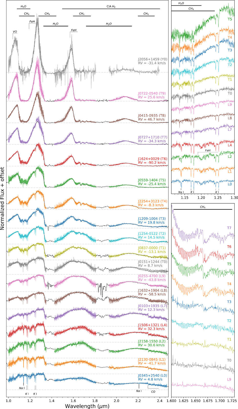
Here are some plots that show an initial S/N estimate exercise. Given that the background tends to kill you in slitless spectroscopy, compact sources (PSF) are great.

Anyone who wants to play with S/N matters, go to the collab notebook here

This shows at R=1000, 1.5mum the continuum S/N (per resolution element) in a 1000 second exposure for sources of different spatial extent, as a function of their size (source diameter)

This shows the S/N (per resolution element) for a continuum point source, as a function of telescope diameter. For reference, Euclid~1m, Roman~2.4m

This is an analogous plot, but for a (spectrally) unresolved emission line on top of negligible source continuum. The envisioned line-flux sensitivity for ground-based "stage 5" redshift experiments (0.5e-16) is indicated (see https://arxiv.org/pdf/2209.03585.pdf )

This is a first attempt at mapping the S/N to some physical input, such as a star-forming region/galaxy as a function of of their size and SFR. Yes, spatial extendedness is a killer.

=======

Reminder 1: what is the physical resolution as a function of redshift

=======

Just as background, here's the sky values from Rigby+2023

Science Cases with such a Survey:

This deserves simulations and asking what range of lambda,R,NR, etc.. is optimal, and which acceptable

Spectra of Stars:

• 2-5 abundances of cool stars
• are there any zero-metallicity stars in the Milky Way?
• chemical identification of streams (as small-scale DM probes)
• find the fastest stars (in the bulge): BH dynamics
• spectra of every O stars within 5 Mpc
• free-floating (semi-young) planets and stuff

Spectra of AGNs:

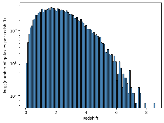
• AGN as LSS probes to z=7(?)
• earliest AGN (z~12) ==> BH growth; seed BHs

Spectra of Galaxies 

What can we expect for emission line spectroscopy of galaxies?

Let's take the Yung, Somerville+2022 SC-SAM simulations, and the Kennicutt

conversion of SFR --> Halpha; and request a 7 sigma Halpha detection, given line flux and disk-size of the galaxy. Consider a total area of 10.000 sqdeg on the sky. Quite staggering galaxy numbers ....

• ?? <what are the most interesting things>
• host galaxy diagnostics of BH GW events with LISA

Cosmology:

• probes of inflationary signatures (by stage 5+ spectroscopy)

• kinematic lensing on steroids
• 
  

(inadvertent) Spectra of Transients

• way too many gravitational lenses with spectra
• serendipidous (single epoch) SN spectra to faint levels
• GRB hosts
• tidal disruption events in AGN
• <you name it>

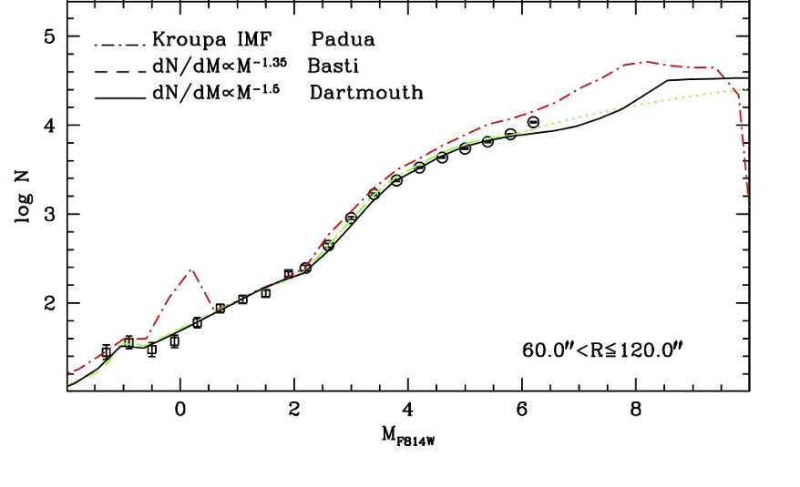
Low-mass objects

• there are ATMO2020 models from Phillips+2020 and newer (JWST-oriented) models Legget&Tremblin 2024
  
  
  

from Theissen, Burgasser et al 2023.  LTY dwarf spectral library

How many more stars (for stellar streams) does one get going below the MS turn-off
(from Bellazini+ https://arxiv.org/abs/1203.3024) 

going from absmag 2 (in I) to 3 is 20x more stars

Notes on crowding:

I downloaded Gaia data in Baade's window, and did number counts, which resulted in an estimate of how many stars there are per spectral streak area (code at getBaadesWindow.ipynb) in 

/Users/rix/Science/Projects/SlitlessSpectroscopySpace/SpectraSims

The plots looks like this, and implies that the crowding is unproblematic to 21st magnitude

Next steps would be to 

a) get deeper data

b) calculate the Poisson probability of being uncontaminated and add it to that plot.

More science application ideas

The universe through a looking-glass

Strong (>30) lensing magnification (size and flux) happens, by is rare. When it happens, it opens up a new regime of spatial resolution.

Takahashi et al 2011 have calculated statistics. The plot below shows magnification averaged over 3kpc

For compact sources there should be much more magnification.

Extreme magnification probabilities have been discussed in Diego (2019)

So, there is a 1 in a million chance to get magnification of more than a 1000. A linear magnification of 20 leads to a physical resolution (6.5m at 0.75mum) of 9 pc at z=5.

Possible next steps in XP spectra & the Milky Way

 These are literally only notes-to-self by HW

The Rich Heart of the Milky Way

[see also the Jupyter notebook: Metal Rich Stars from Andrae+2023]

I just made the plot using the Andrae+2023 giant table

We can then identify the most metal-rich stars in it [M/H]>0.47.

Their CMD's look "normal"; but iffy [M/H]-estimates and imprecise parallaxes

prevent clear age-dating.

We then look at the all-sky distribution, in different metallicity slices, which looks remarkable

 To do's:

• plot [M/H]_XP vs DR17 APOGEE - get new metallicities from Andy Casey (?)
• check whether there are any RV's (few?)
• get good distances (a la Hogg...) or from Xiangyu
• with good/assumed distances, say something about the ages
• build a model to constrain the level of rotation using only proper motions (that needs good distances). -- get proper motions!! (the notebook is set up for that)
• all this requires a clean-up/augmentation of the Jupyter notebook.

Giant Ages within 3 kpc

For giants with XP metallicities and very good parallaxes (5%?) we can get ages, as in the LMC, using HWR's sped-up code.   We should do that..  perhaps suggest to to Josh?

Calibration of the stellar mass scale on the lower MS

I have taken the Hwang et al 2023 code that calculates (and dynamically calibrates) M_*(absG,B-R) from the wide-binary dynamics and applied it to M-dwarfs. Compared to the what the Carmenes DR1 folks use, there is a serious offset.

Interpreting the Gaia astrometric orbit catalog: constraints on objects at 2 AU

 "Modelling" the Gaia DR3 Astrometric Orbits (a.k.a. learning astrophysics from complicated catalogs)

The Basic Idea

Gaia has produced many catalogs with constraints on interesting astrophysical phenomena. In particular, Gaia DR3 has produced a catalog of >130,000 "astrometric orbit solutions", where many-epoch observations of a sources have lead to an "orbit".  Specifically, the light-centroid position of the source on the sky can be (well) fit by a combination of parallax, proper motion and a Keplerian orbit.

This catalog (lovingly dubbed gaiadr3.nss_two_body_orbit) should be a treasure trove on questions on how stars deal with their angular momentum during formation (binarity, or planetary system), on stellar evolution (what if one of the stars in a binary dies to become a WD, NS or BH)?

But it turns out that it is not easy to go from "What's (not) in the catalog?" to astrophysical questions such as "How often do low-mass stars have even lower mass companions?"  "How common are giant gas planets at, say, 3 year periods, around stars of different mass?", "How common are brown dwarfs are companions?", or "How often are stars orbiting stellar-mass black holes?"

This  catalog<-->question  link is not easy for a variety of reasons. First, and foremost, no catalog contains everything. It usually (and sensibly) contains what the underlying experiment can detect or measure well. Second, acknowledging this incompleteness does not yet help. To learn from the catalog one must build a model that predicts the ensemble of catalog entries, and this model must incorporate the selection function (e.g. Rix et al 2022; and references therein for a recent exposition of this issue). The selection function specifies with what probability (often 0 or 1) an object of any properties (flux, temperature, distance, direction, etc..) would have ended up in the catalog or not. The selection function should be a function of variables that a) are "observables" and b) can be predicted by the model.

 For "literature" samples, the selection function is hopefully specified in terms that lend themselves to modelling; else it may need to be (painstakingly) (re-)constructed. By comparison, specifying a "model" is often easy. E.g. for the scienc e theme discussed above, the model could be given by a single number: what is the probability pJ that a solar-type star in the Galactic neighbourhood has (as dominant companion) a Jupiter-mass object in a 3-year orbit.

To get specific, let's make a plot of the catalog in which the Gaia mission speaks about (astrometric) binary orbits.   There are many things to be plotted about this sample, but the following Figure (showing all 134,000 sample members) cuts most to the chase.

The X-axis shows the inferred period, between 0.1 years and 10 years, with the prominent 'aliasing gap' at 1 year. The Y-axis shows the 'Astrometric Mass-Ratio Function' (AMRF), a clever quantify devised by Shahaf et al. ( 2019 ). It links the light-centroid motion (observable) to the motions of the primary and secondary. If the primary dominates, then AMRF becomes an approximate measure of the mass ratio, q. 

So, interesting companions are either at very high AMRF (black holes, neutron stars ??) or at very low values (planets, etc..).  And, the plot shows very little / nothing at extreme AMRF. What does this mean for the incidence of BH's and planets orbiting stars in the pertinent period range....?

That's the basic issue to be addressed.  

The Basic Mathematics

Let's take as (interesting) toy case that we want to constrain is the rate at which solar-type stars have Jupiter-mass objects MJ in ~2AU orbits. 

This is a special case of the following general model that constrains the probability "p" that a stars of a c ertain mass and metallicity has a planet of Mp in an orbit size "a" and eccentricity "e".

This model is now to be compared to the "data" (which is in essence the set of catalog entries in the "orbit catalog" above).

In addition to the light-centroid parameters ("lc"), we need the parallax (to convert milli-arcseconds to AU), the apparent magnitudes \vec{m} (which set the S/N; see below), and an estimate of the primary star's mass (which comes from other information), as Kepler's law needs that.  The Gaia catalog contains such information for N_*=134,000 stars (see plot above).

The nest (and hard and crucial) step is to understand under which circumstances a system might have ended up in the catalog. Why this is crucial, we'll show below; let's for now just go with it.

For Gaia DR3 the following conditions have to be fulfilled (Halbwachs+2022).

These are S/N conditions on the parallax (varpi), and on the quality of the light-centroid semi-major axis (a_0). There is also a criterion on the eccentricity uncertainty. For operational reasons all these criteria depend on period.

The art, and bain, is to express the selection function S correctly. This function S is the probability that a system with certain physical characteristics -- stellar, and planetary mass, distance, period, etc.. -- would have passed the selection criteria. We have to be able to go to any (even just envisioned) star of certain mass distances etc., and answer: if that star had a planet of certain mass in a certain orbit, would it have resulted in a catalog entry. 

Initial version of such an approach was worked out in El-Badry+2023, for the regime of massive dark companions); there it seemed that the parallax/S/N criterion was the most stringent. If we assume that the parallax uncertainty is (mostly) a function of parallax, brightness of the stars and semi-major axis of the orbit, then we can make the selection function a relatively simple function of "model-predictable observables" [More to say here].

This then leads to the following prediction of how many systems we should see in the catalog:

How to interpret this? To predict the number of catalog entries that imply a planet of mass M_p in an orbit of size a -- for a given model p(M_p,a) -- we need to sum over all stars (yes, ALL stars) and sum up their selection function.  Of course the sum over all stars is silly, as for almost all stars in the Milky Way the selection function probability is S==0. So, in practice, it boils down to counting all stars in the catalog for which S==1 (in a given dM_P x da ) and comparing that to the number of actual catalog entries (using the binomial statistic). 

The delightful aspect is that -- once the selection function is specified -- the exercise becomes "trivial".

Selection Function Nitty-Gritty

<here we'll eventually spell out how to determine and then apply a suitable selection function>