(variability-based) YSO selection for SDSS-V

Starting point

In the previous post I made a proposal on how to select (low-contamination) samples of YSOs for SDSS-V targeting, through a combination of WISE W1-W2 excess, variability, and a parallax cut to eliminate backgrounds. This was based on:
YSO's can be discerned by (any combination of) the following observational properties:1)  their SEDs (0.5-20mum) are not-just-a-simple-photosphere (..disks, accretion, etc..)2)  they lie off the(ir) main sequence3)  many (most?) of them show some flux variability
4)  they are clustered in position and velocity space.

This (at first glance) seems to do very well at selecting YSOs (Class 0,I,II) that a) have a mid-IR excess (W1-W2>0.25), and are bright enough to show up in the Gaia catalog (G<18). But that leaves out later YSO phases (no W1-W2 excess), and thereby leaves out objects (Class III) that a portion of the SDSS-V YSO group care about. 

Here a propose a considerably broader YSO selection for SDSS-V (which encompasses the above approach), which is largely based on optical variability, but still seems to get low-contamination samples, though are more dominated by more 'mature' (low-mass) YSOs. To keep background contamination in check, the sample distance needs to be limited (e.g. to ~1kpc). Which subset of these YSOs are interesting enough to get targeted in the SDSS-V context needs to be sorted out.

The overall approach can be summarized as:

[ Gaia-detection (var>0.0x mag)  or  WISE-color-excess-Gaia-non-detections ] AND H~<12

where Gaia-detection may mean G<18 and parallax>x mas (x=0.3-1.5).

Variability Selection

Selection "Philosophy"

We are seeking YSOs that are a) bright enough to be well within Gaia's flux limit (G<18), b) are bright enough in H-band to be sensibly observed within the SDSS-V context, c) and are YSO's in the sense that they have not yet reached the main sequence of their Minit.
"Variability" in Gaia DR2 is defined as sqrt(g.phot_g_n_obs)/g.phot_g_mean_flux_over_error  i.e. via the photometric excess noise.

Query

I run on ESA's Gaia DR2 server, with a distance cut at 1kpc (TDB, g.parallax - g.parallax_error > 1) ; 

SELECT  * , sqrt(g.phot_g_n_obs)/g.phot_g_mean_flux_over_error as variability

FROM gaiadr2.gaia_source AS g

INNER JOIN gaiadr2.allwise_best_neighbour as xaw

    ON xaw.source_id = g.source_id

INNER JOIN gaiadr1.allwise_original_valid as allwise

    ON xaw.allwise_oid = allwise.allwise_oid

WHERE

g.phot_g_mean_mag < 18.

and

sqrt(g.phot_g_n_obs)/g.phot_g_mean_flux_over_error > 0.02

and

sqrt( g.astrometric_chi2_al / ( g.astrometric_n_good_obs_al - 5)) < 2.

and 

allwise.w1mpro < 12.5

and

g.parallax - g.parallax_error > 1.

See  here for an explanation of the query "philosophy".  I subsequently make a cut to H<12.5, and excise sources with W1_error or W2_error > 0.05 (TBD: is this necessary?).  I also run -- on a subset of the sky -- the exact same query, just insisting that variability < 0.02.

This yields a set of 93.000 stars; query output (i.e. "the sample" is here as a fits file).

The following Figure shows the distribution of this sample in the mid-IR excess (W1-W2) vs variability space. There are three regimes: W1-W2>0.25 (Class I,II objects), a group of low-variability objects at W1-W2~0.1, and the dominant plume at W1-W2=0 (stellar photosphere only?).

W1-W2 vs variability (for H<12.5, D<1kpc). Three regimes are apparent: sources with mid-IR excess (W1-W2>0.3);  (the dominant subset of sources with simple "photospheric" colors (W1-W2~0), and the (low-mass) sources with W1-W2~0.17.

CMD Distribution of Variability Selected Stars

Obviously, youth or YSO-ness is not the only source of >0.02mag variability among stars within 1kpc, they pulsate, eclipse, etc.. I certainly had no idea or preconceived notion of which fraction of the H<12.5 D<1kpc var>0.02mag stars may be YSO. The availability of parallaxes allows us to put these stars onto a CMD.

Let's stars with looking at the complementary set: (a subset of) stars H<12.5 within D<1kpc that does NOT vary (at the rms 0.02mag level):

Non-varying stars (at <0.02mag level) with H<12.5 (G<18) and D<1kpc(plx>1mas). Overplotted are (Padova) isochrones of log(t)=6.6 -- 9.6 in steps of 0.5 dex (4Myrs,12Myrs,40Myrs, etc..); this all looks nice and "boring".

Once can see a hint of the binary sequence, but otherwise this looks like a 3-10Gyr old population (to me). As expected, the combination of geometric survey volume and magnitude limit, prefers a certain stellar luminosity (those still bright enough to make the magnitude cut at the maximal distance).

Now let's look at the analogous query, but ALL stars that vary by variability>0.02mag.

Stars H<12.5,D<1kpc and variability > 0.02. The vast majority of them lie above the MS!

The following is the same plot as above, increasing point size to show that all the very reddened YSOs are still in here...

As above, but showing the sparse parts of CMD space.

Remarkably, the vast majority of these stars lie above the (old) main sequence, around the 4-40Myrs isochrones.  That patterns becomes even more distinct, if we look at the stars that vary by at least 0.05mag rms, as shown here; insisting on larger variability also selects against low-mass YSOs (?).

As above, but restricted to stars varying (rms) >0.05mag.

If that is true, then the majority of stars (H<12,D<1kpc) that vary by 0.02mag (or certainly 0.05) mag are YSOs (??!!??). Can someone educate me whether that can be true?

Obviously, this sample include all kinds of other variable stars, but they seem to be a modest fraction.

-------------------------------------------------------------

Aside: Variability Selection in the Orion Region

If I take I select all stars form Gaia (G<18.5) within 190<l<215 and -26<b<-8 and 2<parallax<3,

I get this

I can now split this in the non-variable sources (variability < 0.02mag; 53.000 sources)

and variable ones (variability > 0.02mag; 7000 sources)

and those 2000 with variability > 0.05

And now an aside on the aside: this is all for PMS stars (in Orion absG>4-ish). The more massive stars in Orion (absG<3, parallax and PM selected)  that have presumably reached their MS show no variability:  shown as larger symbols (color-coded by variability) on top of the lower-mass var > 0.02 background.

Seems all pretty neat.

[end of aside] -----------------------------------------------------

On-Sky (and Parallax) Distribution of these Stars

If that interpretation is correct that variability >0.02 is an efficient (both reasonably complete and pure) YSO selector, then this should be reflected in the sky distribution.

Let's start with the "easy" case: 2300 YSOs with distinct W1-W2 excess (>0.2) (and H<12.5 and D<1kpc) shown as a sky map woth parallax as color-coding.

W1-W2>0.2 stars within 1kpc that have H<12.5 and D<1kpc.

As above with larger dot sizes to show the correlation between position and distance.

This seems to give a very clean sample, as before here , just restricted to D<1kpc.

Let's now contrast that with the control sample that has no (<0.02mag) variability.

.. a nice smooth on-sky distribution, with most stars near the geometric sample limit, 1kpc.

Now what about the stars that have no W1-W2 excess (actually all variable stars, most of which have not W1-W2 excess). Their sky distribution looks like this (var > 0.02mag)

Alls stars (H<12.5, D<1kpc) that vary at >0.02mag, color-coded by distance. The two vertical features must be data artifacts.

and like this when restricting to var > 0.05mag, or like this

Question: what is that warped configuration? Gould's belt? I have no idea... Tell me what paper to read.

when restricting to D<500pc.   If we take the subsample with small mid-IR excess (W1-W2~0.18) the sky distribution looks like this:

Again showing the stronger spatial clustering of younger objects. (my conjecture)

Next steps verification:

My current conclusion is that variability alone is very effective at picking out objects too young to have settled on the MS of their mass. If this is a useful definition of YSOs, then most of them are YSOs. The ones with strong mid-IR excess (W1-W2) are very tightly clustered. The ones with W1-W2=0 and low-variability (0.02-0.05mag) have a considerably smoother sky distribution. If many of them are 30Myr+ old, this may not be surprising.

Questions to all: 

1. What needs to be done to verify this?
2. What's the interest in young (PMS) "field" stars?
3. Please pay with the query results, as a proposed sample file to draw from. ( https://www.dropbox.com/s/de832x5p78q6y8h/GDR2_var%3E0.02_H%3C12.5_G%3C18.fits?dl=0 )
4. What's the best way to augment all of this by WISE-selected (Class I) sources, that don't show up in Gaia, but have H<12? Of the MANY towards the Galactic center, which are interesting? 

==============================================================

Another aside on: which sources does a simple criterion W1-W2>0.25, H<12 select, and of these, which sources is a Gaia variability selection missing? 

And, is it enough to get all the ones that have H<11 through the GalacticGenesis program anyway? [Should those get a priority flag?] The plots below show ALL W1-W2>0.25, H<12. sources.

Here is an approximate map of those sources that are NOT in Gaia

and here is their galactic latitude distribution quantified: they are almost ALL exactly in the Galactic plane.

I.e. there is a modest number of such (missed sources, not in Gaia 11<H<12) sources in Orion, but the vast majority  of them are inner disk (within 1deg of the Galactic plane). What should we do about them?

Let's look at the Orion region, defined as

There are 1127 sources that pass H<12 and W1-W2>0.25. Of those, 1085 (97%) are in Gaia, and 979 (87%) bright enough to be included in the variability selection. Do we need to address those?

end of aside
====================================================================

Implications for SDSS-V target selection:

This picks out nearly 100k YSO/Young stars targets, which is more than we can target. 

 My proposal for SDSS_V YSO targetting: let's make the sample definition:

-- all stars with H<12.5, and W1-W2>0.25 and D<5kpc

and

-- all stars with H<12.5, variability>0.02mag  and D<1kpc

Or put differently:

-- all stars with H<12.5, variability>0.02mag  and D<1kpc

augmented by 

-- all stars with H<12.5, and W1-W2>0.25 and 1kpc<D<5kpc

Implicit is G<18, and we then need to set a targeting priority, where priority decreases as  W1-W2 decreases. E.g. if "second priority" are the targets with slight W2 excess, we still zoom in on clusters.

YSO selection for SDSS-V

Towards defining YSOs targets for SDSS-V

Science goals:

Previous post, dealt with identifying samples of stars that are massive (>5M_sun). I'd like to explore what can be done interms of an "algorithmic, all-sky" sample definition for (lower-mass) YSOs.

YSO's can be discerned by (any combination of) the following observational properties:
1)  their SEDs (0.5-20mum) are not-just-a-simple-photosphere (..disks, accretion, etc..)
2)  they lie off the(ir) main sequence
3)  many (most?) of them show some flux variability
4)  they are clustered in position and velocity space.
5)  dominant selection contaminants are dust-reddened giants of various sorts.

To start, I took a simple stab at combining the aspects 1), 3) 5)  Basically, I tried to find the objects that have YSO-like WISE colors (i.e. W1-W2 significantly > 0), that vary on year-timescales by a > few percent, and are within 5kpc (to cut out background). 

What I do requires some detection in Gaia (for starters I took G<18);
this clearly will miss seriously embedded sources.

This approach uses two aspects of Gaia that are perhaps non-obvious:
-- already now, Gaia is a high-precision, all-sky variability survey: 

    at the moment one gets only the rmsvariability amplitude
    on timescales of a year, encoded in variability == sqrt(N_obs)*flux_error/flux 

    (needs correction at the faint end).
-- and while the parallax measurements for such WISE-color-selected samples 

   will be insignificant for much of the sample,  plx/plx_error < 1, this is still very   

 informative: e.g. at plx_error < 0.2mas, plx/plx_error < 1 means you are NOT nearby.

Having said that, I queried GaiaDR2 x WISE for  

 variability>0.05mag,W1-W2>0.2, Gaia_G<18  and no astrometry flags.
When plotted in WISE color space (excising bad W1 and W2 photometry, 

left-nad panel)  this selection yields 26.000 objects:

Stars selected by variability>0.05mag,W1-W2>0.2, Gaia_G<18

These stars have an interesting distribution in variability amplitude.

Then I sub-select the objects that lie within 5kpc from the Sun (at least at >1sigma confidence),
i.e. parallax - parallax_error > 0.2mas; this is eliminate background; indeed, this cleans the large majority of objects, leaving only slightly over 5000.  In WISE color space,  this leaves a distinct population (the blob around (1.7,0.6):

Subsample from above, selected to be within 5kpc

If I then plot the objects surviving this simple procedure on the sky they look pleasing to my eye
(color-coding is the distance ), when trying isolate a sample of YSO within 5kpc:

This is the on-sky distribution of the stars, selected as above, color-coded by distance.

with a zoom-in on the Orion region (different distance color-scheme)

What seems good to me is:
1) the prominent nearby SF regions are there;
2) there is no apparent bulge/disk contamination;
3) the parallaxes indicate little contamination (i.e. patches in (l,b) have very similar parallaxes); note
that except for requiring parallax - parallax_error > 0.2mas, parallaxes have not entered the selection.

The query that created the sample is:

SELECT * , sqrt(g.phot_g_n_obs)/g.phot_g_mean_flux_over_error as variability
FROM gaiadr2.gaia_source AS g
INNER JOIN gaiadr2.allwise_best_neighbour as xaw
    ON xaw.source_id = g.source_id
INNER JOIN gaiadr1.allwise_original_valid as allwise
    ON xaw.allwise_oid = allwise.allwise_oid
WHERE
g.phot_g_mean_mag < 18  /* magnitude cut, so that variability at 0.05mag can be established */
and
sqrt(g.phot_g_n_obs)/g.phot_g_mean_flux_over_error > 0.05/* variability selection rms > 0.05mag */
and
sqrt( g.astrometric_chi2_al / ( g.astrometric_n_good_obs_al - 5)) < 2. /* weed out bad astrometry */
and
allwise.w1mpro - allwise.w2mpro > 0.25  /* stay away from the boring-star-locus in WISE */
and
g.parallax - g.parallax_error > 0.2  /* stars that are within 5kpc; to weed out background */
Comments in blue must be removed before the query runs

[I did do poor-WISE-photometry-cleaning afterwards]
The resulting output file can be found at:
https://www.dropbox.com/s/1ylqx7c9f4kmkbd/YSO_subset_v2_of_var%3E0.05%3EW1-W2%3E0.25.fits?dl=0

Next steps and action items for the working group:

Obvious limitations:

By construction, the above procedure only selects YSOs with W1-W2>0.25 and G-band variability > 0.05mag, and G<18; i.e. YSOs that do not show significant "W2 excess" and lie near the normal stellar locus, and those that don't vary (by 0.05mag) will not be captured; and those
with Gaia-G > 18. The first aspect means that Class-III objects and more mature PMS phases (sorry about the term) will be missed; the second aspect means severely reddened Class 0 objects will also be absent. This may, will and can lead to an augmentation of the above query.

For such objects, their variability and their position in the CMD must play a larger role; I have started to explore this, and will post next.

Verification steps:

-- do known YSOs, whose established measurements should satisfy the above criteria, show up in the sample? Does the query pick what it purports to. I.e. what falls through the cracks because of crowding, but would still make a good fiber target?

-- what is the overlap/mismatch with established catalogs?

-- can we use existing spectral surveys (incl. SDSS-IV) to verify the purity of the selection?

Orbits and abundance patterns, based on many-abundance LAMOST DR4 (Maosheng Xiang)

Starting point:

The GALAH-label-transferred LAMOST DR4 data set is the (by far?) largest set of stars in the Milky Way with multi-element abundance information. [Of course, only to the extent that the labels can be trusted; see previous post]

Johanna Coronado has augmented this sample of >5M objects with action estimates she did that primarily to look at the correlation of abundances and detailed orbit structure in the Solar neighbourhood. But the sample should also be very good to look at the non-disk components of the MW. In particular, the population of 'inner halo' stars in very radial orbits (sausage, Enceladus, PEM=presumed-early-merger) bear a closer look. This is something that Yua-Sen Ting and Maosheng Xiang may want to pursue as an 'application of the data set'.

All subsequent points were done using a) a sample of 'giants' and b) 'MS stars', just to get at least one test on abundance-robustnes..

First glance intriguing results

Here are some issues to follow-up:

I isolated the set of "stars on slightly-counter-rotating, radial orbits", by picking all stars with
-0.4 < "Lz" < 0.1, where Lz is the normalized angular momentum "Lz" == Lz / (8kpc * 220 km/s);

and asking that these stars are at the same time on highly radial orbits,  sqrt("JR")>0.6, where
"JR" == J_R / (8kpc * 220 km/s).

If we look at the abundance abundance distributions of (only) these radial-orbit 'halo' stars (about 8500 giants, and 6500 MS stars), we find (always "radial orbits" first, then "all orbits").

For Magnesium:

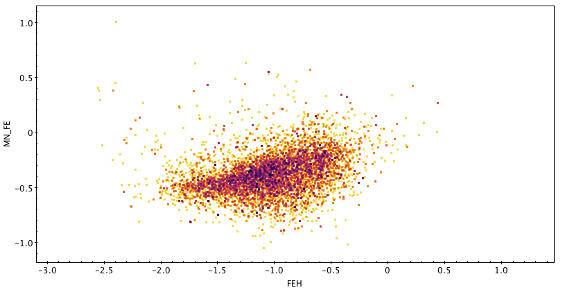
For Manganese

 

For Aluminum:






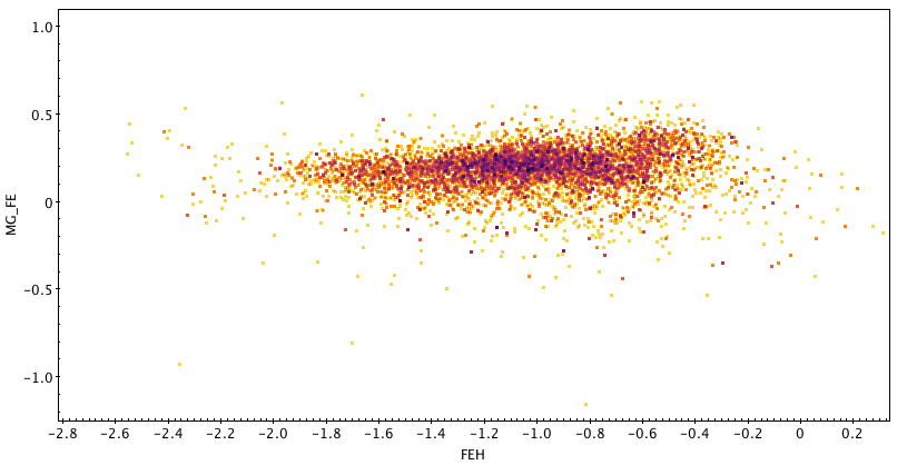
For Europium (can we believe LAMOST from-GALAH-label-transferred Eu?)

in every case, the stars on highly radial orbits are just one striking feature of the overall abundance distribution.





The 'halo' below FeH<-2 looks different; but (see last post) we need to see whether this is an artifact of the abundance analysis.

Next steps 

These plots bring up many questions:

1. Is the "tight" abundance feature -2<FeH<-0.7 a consequence of the label-transfer? E.g. if there are only 20 GALA stars in that regime that show no [X/Fe]-spred, then this is what we expect.  
2. Do we now have a large-sample, many-abundance handle of Sausage/Gaia-Enceladus? How much larger is this sample than others? 
3. Do the abundance trends that we see make astrophysical sense (esp. in the context of the trends expected for a mid-sized satellite galaxy)?
4. The plots for dwarfs look analogous, but do not extend below FeH<-1.4. HWR suspects that this is because there are no very metal poor MS stars in the label-transfer training sample.

verifying the label-transfer GALA --> LAMOST DR4

Starting point

Maosheng Xiang und Sven Buder identified a GALAH DR2 - LAMOST DR4 overlap sample that allowed to attempt a many-label transfer, using Yuan-Sen Ting's data-driven, physical-prior-constrained Cannon-Payne hybrid. That resulted in 6.3M LAMOST objects with assigned labels:

Initial diagnostic plots

HWR made some initial plots, that basically showed that 

1. in many cases everything looks plausible
2. there many spectra where the assigned labels (even the stellar parameters) must be spurious, for a number of reasons. The two main ones are:
1. there are LAMOST data problems, such as 'no blue spectra', etc...
2. Action on Maosheng: put a flag on all objects, where there are serious data problems the labels fall outside of the training range. This is illustrated here (6.3M LAMOST labels in grey; training set as colored dots)



The immediate reaction is to restrict all subsequent science analyses for the time being toobjects that fall within the training range.  [Neige Frankel raised the important point that not all LAMOST objects whose labels fall within the training range, have 'true' labels within that range'.  This may be illustrated with the following diagnostic plot from the low-metallicity regime:

Seemingly, most giants with FeH<-2 have poor chi2; possibly because the label-transfer interpolator cannot predict spectra well that are essentially featureless. That brings up instantly the question of whether the poor chi2 at FeH<-2  systematically distort their FeH estimates

Next Steps

On the verification, most of the next steps are actions on Maosheng. Those steps include:

1. describe how (before the label transfer was done) the input labels were pushed to the isochrones, using Gaia information. Was that done? Is the approach published, else sketch it.
2. devise and implement the flagging (or excising) of 
1. 'bad data'
2. find algorithmic ways to identify spectra, whose label estimates may be distorted as a consequence of label-transfer extrapolation. There may be two ways: either split the training sample in half, and then make two predictions for extrapolated objects (i.e. pseudo-crossvalidation beyond the training set regime), ask how consistent the estimates are; or use chi2, which works in some ways, as this plots shows [color = log(chi2)?]



3. Think about enlarging the training set. Specific proposal include:
1. boost the overlap sample, e.g. by requiring that only logg,Teff,FeH,MgFe,(a 'few' others) are well-measured in GALAH
2. Augment the training sample by synthetic, ab initio spectra (conceptually troubling, eh?), especially in the regime of hot stars (Kurucz Atlas models) or very metal poor stars FeH<-2 (see issue above.)
3. Think about where we can get training labels of very cool MS stars (<4200K) from 

color-selection of OB stars

How to get a simple query criterion to select massive stars in SDSS-V?

Approach:

Find a locus in color-color space that contains hot stars (reddened by different amounts);

Then use Gaia parallax information (NOT: good parallaxes) to weed out all stars in this
color-color-locus that are inconsistent with being luminous (absK<0), or too faint to
be SDSS-V observable mH<12.

At the end, we need to see how complete and contaminated such a sample is.

Starting point: 

take a sample of W1mag-luminous stars from GDR2 x ALLWISE (courtesy Alcione Mora)

(all stars absW1 < -2, or so) and look at them in some color-color space. Below, the Y-axis is chosen to be constant under reddening.

There is a distinct 'plume' in the bottom left, which is (conjecture) reddened blue (massive, luminous) stars, while the mass of objects around (4,0.4) is luminous giants, AGB stars etc.. This is verified by comparison with the literature catalog of Galactic OB stars https://heasarc.gsfc.nasa.gov/w3browse/all/galobstars.html (green points).

Possible Implementation:

We must not rely on "good parallaxes" in any query (as they are usually not available); instead we query on sensible initial 2MASS colors, and only existence in the Gaia catalog (G<21), nothing else

SELECT        g.source_id,g.ra,g.dec,g.l,g.b,g.parallax,g.parallax_error,g.pmra,g.pmra_error,g.pmdec,

              g.pmdec_error,g.astrometric_n_good_obs_al,g.astrometric_excess_noise,g.astrometric_chi2_al

              ,g.phot_g_mean_mag,g.phot_bp_mean_mag,g.phot_rp_mean_mag,g.phot_variable_flag,g.teff_val,g.a_g_val,

         tm.j_m,tm.j_msigcom,tm.h_m,tm.h_msigcom,tm.ks_m,tm.ks_msigcom,g.phot_g_mean_mag - tm.h_m AS g_min_h 

FROM gaiadr2.gaia_source AS g

INNER JOIN gaiadr1.tmass_best_neighbour AS xmatch

ON g.source_id = xmatch.source_id

INNER JOIN gaiadr1.tmass_original_valid AS tm

ON tm.tmass_oid = xmatch.tmass_oid

WHERE  b between -15 and 15

and

tm.h_m - tm.ks_m -0.48*(tm.j_m - tm.h_m) between -0.12 and 0.5

and 

tm.j_m - tm.h_m < 0.8

and

tm.h_m < 12.5

This yields (in an analogous color-color) plot a hint of bimodality (with hot stars bottom left plume, again) ...  but these distributions (1.7M stars) are mushy.

We now excise all stars where Gaia information tells us that they are inconsistent (at say 1 sigma) with being luminous, absK< 0, (i.e. OB stars) (After 7Myears, H<0 corresponds to M>5M_sun; Padova isochrones, is that correct?). Effectively this does a ``forground clean".

kmag + 5log10(parallax+parallax_error)-10 < 0. This leaves 0.6M stars (i.e. 1.1M stars excised).

Note again that Gaia only comes in in two ways:

-- there must be some detection (G<21-ish)

-- and Gaia parallax measurement (however 'lousy') must not be inconsistent with this being a luminous star.

This yields a nice hot-stars r-- red giant/AGB bimodality; showing that the color-color locus of reddened hot stars is distinct from that of RGB, RC, AGB etc. stars. This is illustrated again by comparison with literature OB stars (reference above)

Taking the lower part of this bimodal distribution leaves ~75k candidates M>5M_sun and m_H<12.5; they are very much concentrated to the Galactic plane; the stripy pattern is Gaia scanning law....

Data at: https://www.dropbox.com/s/ogxmtxag05slkeg/initial_JHK_color_cut_consistent_with_K%3C0_J-H-W1_color_cut.fits?dl=0

Clearly all this needs verification, clean up etc.. but that's what I mean by algorithmic selection.

A few notes:

-- need to check how good or bad this initial strawman selection is

-- this could be done in a single query

-- we should understand why the bluest stars from the literature are being missed (Rigel too bright etc..)

-- the bimodality-based sample-selection should not be done by hand as here

-- when challenged, I could do the same for low-mass young stars; but I leave this to experts.

Identifying RC stars in Gaia data, and making 3D or 6D maps with them

From YST: can you remind me how do you infer the distance modulus is phot_g_mean_mag+1.27-1.5*bp_rp ? I always thought distance modulus is apparent - absolute magnitude. In other words, why 1.27-1.5*bp_rp is a good approximation for g band absolute magnitude?

Qualitatively, this is based on the fact that RC stars are remarkably good standard candles
in the near IR, say W1. Then you can ask, can I predict the W1 apparent magnitude from
phot_g_mean_mag and bp_rp, combining the effects of effective temperature spread
and reddening: and phot_g_mean_mag -1.5*bp_rp+ const. is the answer.

Then operationally you can take the RCs in APOGEE (which have a range of temperatures
and reddenings, and [Fe/H]..) and ask

what constant (and what bp_rp slope) to I need to predict the parallax (not the distance)
for the whole sample:
varpi_predicted = 10^ (  -(phot_g_mean_mag -a * bp_rp + b  - 10)/5)
and solve for a and b in a chi2 sense (varpi_obs - varpi_predicted)

Then you can go to clusters etc.. and ask whether there are any Teff,[Fe/H] residuals,
which there seem to be none at the 1% level...

Notes on transformation to Galactocentric restframe

What's the best way to transform to Galactocentric restframe?
We have new pieces of information:
8122pc
proper motion of Sgr A*
we are 25pc above plane (Juric)
and we have radial velocity constraints\

Do we want to write/publish a note on this?