Cosmology in a nutshell

 Minimalist "Cosmology in a Nutshell"

Things "every astronomer should kind-of know"; HWR - very undigested list

Space and the overall evolution of the Universe is described by a metric

• it's the Robertson-Walker metric; cosmological principle puts all interesting stuff into a(t)
• a(t) depends on mass-energy-density of the Universe; and an expansion scale factor H(t); (1+z)~1/a
• a(t), which depends on O_M, O_L, O_R, determines the dependence of fluxes and sizes on redshift, which in turn constrains the "Omegas"

An expanding Universe goes through distinct thermal phases: T ~ 1/a

• there are 10^9x more photons in the Universe, but rho_phot ~ a^-4; while rho_mass~a^-3; the two are equal at z~15.000
• after three minutes, kT ~ DeltaE (proton - neutron) --> He forms
• at z~1300 T~4000K recombination P+e- --> H
• "surprising" in light of 13.6EV <--> 20.000K
• scattering off free electrons (Thompson) disappears --> long-mean-free path
• ==> CMB: photons from "surface of last scattering" elsewhere, reaching us now
• CMB bizarrely uniform on large scales
• small-scale temperature fluctuations (10^-4.5) reflect initial density fluctuations (in complex ways)
• at z~9, discrete UV light sources (hot stars, accretion disks) re-ionize the Universe
• making it (partially) transparent in UV

Structure grows, eventually forming galaxies, etc..

• initial fluctuations seeds in inflationary epoch (frozen quantum fluctuations)
• grow happens in competition between gravitational instability and expansion never faster than linear delta ~ a. <-- therefore structure growth depends on (and constrains) the Omegas
• eventually some fluctuations become no-linear --> gran. collapse --> halos

We now know the Omegas and Ho at the % level

• from all the above

thoughts on new, but potentially misclassified, classical Cepheids (I20+ sample)

On simple lightcurve classification to for classical Cepheids in the context of the Inno+20 draft

Starting point:

We have ~800(?) new classical Cepheid candidates from I+20. A good number of them have been recognized as variables in other surveys, but classified as different sources. The main other classifications are:

a) eclipsing binaries (EB)

HWR's 'by-eye' distillation of lightcurve characteristics that look non-Cepheid-like:

• rise and fall are symmetric; i.e. flipping the time axis would leave the light curve invariant
• the downward deviations (from the median) are larger than the upward deviations

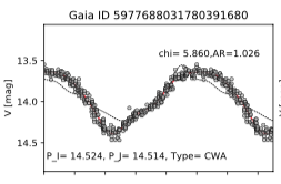
b) W Vir (CWA & CWB)

HWR's 'by-eye' distillation of lightcurve characteristics that look non-Cepheid-like:

• rise-time longer than fall-time (only CWA's); opposite to DCeph
• have not discerned lightcurve characteristics in CWB that look different from DCeph

c) rotators (ROT)

HWR's 'by-eye' distillation of lightcurve characteristics that look non-Cepheid-like:

• Fourier decomposition "wiggly", i.e. much power in the 4th - 7th order components
• scatter of individual points from Fourier fit large, compared to Fourier amplitude; i.e. basic periodicity + much "noise"

HWR's Basic Impression

• Indeed, many of the "new candidates" are different types of variables.
• There should be a few simple lightcurve criteria to add/modify that should greatly reduce the contamination. These are spelled out below.

Possible steps to implement:

Diagnosis:

•  let's re-check whether the 'contaminants' do not lie in funny corners of our current lightcurve-shape space (A21,A31,phi21,phi31) that can be cut at little loss to the DCeph completeness.
• the plot below is from an OGLE paper, and sats e.g. that really most CWA's should lie elsewhere in Period phi21,phi31 space

• Can you make plots a la Figure 3 in the draft, with all the externally confirmed DCeph as pale grey points, and the location of the "new candidates" that are classified as "others" by others as coloreds points (as separate colors, or in separate plots for EB, ROT, CWA & CWB).

Possible simple new light curve criteria

Here is a proposal how to use the 7th-order Fourier representation of the light curve to calculate a few other statistics that may be very effective at weeding out contaminants (at little completeness loss).

Let's call that function F7(p), where p=phase within [0,1].

Let me suggest to calculate from the analytic form F7(p) the following quantities:

• mM: the median magnitude,  so that 50% of the period the source is brighter than mM, according to F7(p)
• sig-mM: the variance < (F7(p)-mM)^2 > calculated over the part of the light curve where F7(p) is fainter than mM; and 
• sig+mM: the variance < (F7(p)-mM)^2 > calculated over the part of the light curve where F7(p) is brighter than mM. [I think in all cases a "primitive" splitting of the period in say 1000 bins, and doing all of this brute force, should be fine.]
• f-mM: the fraction of the period (according to F7(p)) where the magnitude is fainter than mM
• f+mM: the fraction of the period (according to F7(p)) where the magnitude is fainter than mM
• f_rise: that is the fraction of the period in which (according to F7(p)) the light curve rises; and 
• f_fall: .. where it falls
• scatter: the rms of the deviation of the data points from F7(p) (in mag), normalized by the rms of F7(p) itself.
• n_max: the number of maxima that F7(p) has within a period: this should be 1 for smple light curves, but 3-5 for wiggly ones. 

So, that seems like a lot; but let's just explore them right now.

I think this is better than "machine learning" classification, because it depends less on the "data quality" the sampling rate etc..

Here's my propsal what to look for in diagnostic plots:

• weeding out EBs:  plot  ( sig-mM / sig+mM ) vs f-mM, for verified Cepheids and verified (or externally classified) EBs. I would suspect that for EB's ( sig-mM / sig+mM )  is greater than for DCeph, and f-mM is smaller; this does not yet capture the time-symmetry of EB lightcurves
• weeding out rotators:   plot scatter vs n_max (as defined above); I would suspect that for rotators scatter and n_max are larger (for DCeph vs ROT)
• weeding out CWA: plot f_rise vs phi21  for DCEPH vs CWA/CWB

Stellar Astrophysics from TESS Lighcurves of Eclipsing OBA stars?

OBA Stars physics from eclipsing light-curves?

Background and Goal

Massive stars, according to conventional wisdom, frequently are in close binaries, of comparable mass (size). First strand: massive star physics is not well constrained, and massive binary structure/evolution physics rests on small samples (10's).  Second strand: detailed lightcurve modelling of eclipsing binary systems (given TESS-like quality) can yield very detailed information 

about Mass (ratios), radius (ratios), Temperature (ratios), etc..

Starting Point and Sample

Eleonora Zari devised a large (500k) sample of plausible OBA stars candidates (G < 16), for spectroscopic follow-up with SDSS-V. Multi-epoch BOSS spectra. The stars were selected to have (intrinsically) blue colors, albeit possibly subject to dramatic reddening, and a likely M_K < 0.

But their variability can be assessed with the usual trick of backing the rms lightcurve variability pout of the GDR2 "errors" (in G, BP and RP).

OBA star candidates in the variability vs color-variability plane. Among blue, luminous stars there are essentially two categories of variables (rms G-band > 0.05): pulsators (RRL & Cepheids), with BP/RP variability ~1.6, and (presumed) eclipsing binaries (with BP/RP~1). The latter are the objects of desire here, and selected as in the Figure below.

The rms of the light curve for eclipsing systems is a funny thing: it dramatically favours systems where the eclipses are both deep and occupy a substantive fraction of the orbital period: very close, equal mass/radius binaries are the posterchildren..


Their sky distribution suggests that they are young (massive?) stars:

mostly in the Milky Way, but also in the LMC; the sample if candidate close-eclipsing-binaries contains 1350 targets.

Lightcurve analysis

Their apparent magnitude distribution suggest that > 500 of them should be in the TESS lightcurve 'comfort range'.

But their sky distribution implies crowding that might affect the light curve quality.

Does it makes sense to check for how many of them TESS light curves are available? And then fit them?

pseudo-wide-area-IFU: slit-less bright stellar spectroscopy

Mapping stellar pops/kinematicss with slit-less spectroscopy?

Science goal:

There are parts of the sky that are quite 'crowded' in stars, where we would like to get some basic spectroscopic information for all (bright enough) stars: velocity, Teff, (logg), and [Fe/H] (other elements, too?).

The prime example (accessible to optical observations) in our Milky Way may be Baade's window; and parts closer to the Galactic center, for near-IR observations.

This would lead to orbit-abundance-age(?) information for vast sets of stars, as a basis for dynamics,

and for formation studies based on the structure of the abundance-orbit distribution.

Effective ways of getting such information:

The "obvious" straightforward approach may be to do vast bona-fide IFU mosaics. But this approach is likely to hit its limits (sociological, time-allocation?) at 100-200 pointings? At any rate, e.g. Baade's window is 1000's [TBC] of squarearcmin (or MUSE FOV's).

Slit-less spectroscopy as an alternative?

The basic set-up envisioned is a follows: consider a classic long-slit spectrograph, where usually a slit selects a tiny fraction of the focal plane for subsequent dispersal by a grating/grism/prism; often a pass-band filter in the optical path limits the spectral extent.

Now, envision that same set-up, but with the aperture (slit) plate removed. Let's consider the regime of a single bright star in the field: the detector then will show a simple spectrum of this star; as the star is a point-source, the slit mainly served to eliminate much of the sky background. So, one will have a spectrum of a star (limited by, say, a narrow-ish passband filter of, say 200A), but with "200A's worth of sky", not the "2A's worth of sky" (for a slit).  Note, that to good approximation, the stellar spectrum depends on 5 numbers, (x,y)_pos, flux, Teff, v_los, [Fe/H]   (where logg and flux are degenerate at a known distance).  If you wanted to get (Teff, v_los, [Fe/H]) for that star, you'd fit model spectra, given (x,y)_pos, flux. These 6 pieces of information are to be compared to photometry, which yields three pieces of information: (x,y)_pos, flux.

Now, imagine the field being full of bright stars, and slit-less spectroscopy. It will look the same as before, just like a seemingly (!) crowded mess with 100s (1000s) of star spectral streaks, many of them overlapping. But -- and this is the core conjecture of this approach -- when it comes to information content, this image is not much more crowded. Let's presume that we have photometry, which makes (x,y)_pos, flux_normalization a "given". Then we have to solve for 

p( { Teff, v_los, [Fe/H]}_(all_stars_in_field) | {(x,y)_pos, flux}__(all_stars_in_field) ).

As long as the signal detection is linear, this is just the linear superposition of the problem above.

And, if observations at different angles are obtained (2-3), then degeneracies of directly overlapping

stars could be mitigated [HWR's view: that's almost unneeded: the famous SB2 binaries show that

separation in velocity space suffices..]

The bain is possibly: how narrow to choose the passband filter., not to get killed by sky; but still have enough spectral coverage to get stellar parameters.

M-dwarf Abundances from LAMOST spectra

Overall science goal:

Get systematic "stellar parameters" and abundances for M-dwarf, who have risen to prominence through the TESS focus/fixation as planet hosts.

My loose definition of M-dwarf is all stars cool enough to show serious molecular features in the red optical.

The thoughts below have in part emerged from discussions with Yuan-Sen Ting, Maosheng Xiang and Doug Finkbeiner.

Devise a way to get such labels for all/most TESS targets by 2023; but this note is only about technique

Stellar Parameters: Ideally we'd like mass, age, ... ; that is conventionally rephrased in spectroscopy as Teff and logg, whose relation for (late) M-dwarfs is not trivial because the Hyashi track takes so long. But in data-driven approaches th eproblem is that we'd need trustworthy training labels Teff and logg which we do not have in the first place.

Proposal: introduce M_K and J-K (or some other absolute magnitude and color) as basic stellar labels; for a sub-set of M-dwarfs these are known exquisitely.

Abundances: there are many ideas about which abundances matter (encased in the photospheric abundances)  for planet formation; let's start with [Fe/H] and then add other [X/Fe]; the target precision of [Fe/H] should be < 0.1dex; else it is not very interesting.

A new data-driven angle at the problem:

Gaia DR2 has given us vast sets of wide binaries (>10"), including a significant number of G-dwarf -- M-dwarf binaries where there are LAMOST spectra for both components. The idea is that we get extremely precise distances to the G-dwarfs, and well understood abundances ([Fe/H] and ~10 more).

As atomic diffusion is a minor issue in cool stars with convective envelopes, we can assume that in a binary [Fe/H](G-dwarf) = [Fe/H](M-dwarf). With photometry for the M-dwarfs that gives us training labels labels= (M_K, J-K, [Fe/H]).

We'll train a Cannon type model f(lam) = f(labels), and then infer in a test step labels for all M-dwarfs with spectra.

Implementation

Many of the LAMOST spectra of M-dwarf in wide binaries are of modest S/N, seemingly unsuited to training a model. So, let'd take denoising measures first.

1. take high S/N M-dwarfs (selected in the CMD from M_K and J-K) and construct a clean PCA; determine how many components are needed to get an excellent representation; let's presume 50 components.    The projection of f(lambda) onto the first 50 PCA components become the new "spectral pixels".
2. Take the M-dwarf spectra in binaries (low-ish S/N) and project onto the 50 PCA.
3. Train a 3-label Cannon on this, and do test step (as the first "dumbest" step)

How to do better? Acknowledge that there may be more latent labels (whose existence for the moment we acknowledge, but whose phys. interpretation we don't care about for now).

1. take the residuals from the steps above, and perform a PCA on them.
2. declare the first few components (K) of this residual-PCA as the Cannon vectors to go with latent labels.
3. Project each training stars' residuum spectrum onto these PCA components, and declare the coefficients to be the (initial) latent labels of the training set.
4. Fit a Cannon for those K+3 labels,... iterate?

Diagnostic plots

The following plots compare the LDR5 sample and its ddPayne analysis to Padvova solar-abundance isochrones, in order to 

a) see how many M-dwarfs have observations

and

b) what the ddPayne does in this interpolation regime?

Note that M-dwarfs start at <3800k div="">

This just shows that low-mass stars take >100Mio years to settle on the main sequence

The current implementation of the ddPayne does not give robust Teff values below 4000K. This shows that there is a vast number of M-stars in the sample (100.000) that TESS folks care about, and about which the current ddPayne says nothing. The file with presumed LDR5 M-dwarfs (selected by their (G-H nd M_H) is here: https://www.dropbox.com/s/fy5je8bdkllczao/LAMOST_DR5_Gaia_WISE_Mdwarfs.fits?dl=0

 This shows (ddPayne Teffs small dots; large dots isochrones) that the ddPayne Teff 'stalls' at 4000K; actually a sensible behaviour.

Same as above, just different color as X-axis.

Here the isochrones are color-coded by stellar Mass.

Interpreting global (stellar) kinematics of the disk, in terms of spirals

Background and Set-Up

Eilers and Hogg have created "global" stellar kinematic map of the Galactic disk, with 6D information on ~20.000 stars extending in RGC from 0 to 20 kpc. Between 6kpc and 13 kpc [TBC]

this map shows nice "spiraly" radial velocity pattern, that we should attribute to a "spiral perturbation". 

The question is what practical ways are to interpret these data in terms of (dynamical) spiral arm perturbation (its strength, pattern speed and morphology). 

These notes hare have emerged from conversations between C. Eilers, J-B Fouvry and H-W Rix in HD, and serve (among other things) to bring D. Hogg in the loop.

The observational information

This "map" is actually n(R,phi,z,vphi,vR,vz) == f(R,phi,z,vphi,vR,vz) x S(R,phi,z,vphi,vR,vz),

where S(R,phi,z,vphi,vR,vz) is the selection function.

The main issue with the selection function is that it separates into

 S(R,phi,z,vphi,vR,vz)=S(R,phi,z) x S(vphi,vR,vz), where S(R,phi,z) = very complex, and S(vphi,vR,vz)=const. The selection function can be writen as S (D | phi,theta)*S(phi)*S(theta), where

R=Ro-D*cos(l) cos(theta) and z=D*cos(theta); S(phi) and S(theta) are highly structured, S(D | ..) is (kind-of) smooth.

Rather than modelling the fill distribution function in action-angle space F(J,theta) [the "other theta"],

we se whether there is a sub-space, where the selection function is flat, taking advantage of S(vphi,vR,vz | D,phi,theta)=const.

The proposal here is to model the radial actions and radial angles; as their experimental selection effects may be benign.

Conceptual modelling approach:

We observed a distribution of stars in the disk, which is approximately axisymmetric, but has significant non-axisymmetries (see above). We would like to link that to a driving non-axisymmetric, time-dependent perturbation, focussing on the region >5kpc, as the pattern speeds are slow enough

that co-rotation (and hopefully other resonances) is 'far out'. [JBF stresses the importance of this!]

The problem of linking a time-dependent, non-axisymmetric potential to the resulting non-axisymmetric distribution function has been essentially (theoretically) solved (in the linear, and  non-self-consistent regime) by Monari & Famaey (2016), building on Section 5.1. in BT.

If one has solved the axisymmetric problem, Phi_0 and f_0, one can write for a small/linear deviation from it:

which then leads to the following select steps:

Propose a periodic (in phi) potential pewrturbation

then

spelled out in cylindrical coordinates

resulting in a (formally) closed solution with:

and other terms. Basically all this is spelled out in MF16.

Conceptually, the miracle is that the explicit time-dependence can be eliminated to a seeming steady-state solution in a co-rotating frame (Eq 15 --> 16 in MF16).

Implementation issues:

Here are some suggestions (to Christina) how to implement it:

-- go through the Monari&Famaey paper and re-write/simply it to the 2D case of a razor-thin disk;

    probably a good idea to wrapy your mind around the math.

-- let's choose a very simple Phi_1 perturbation functional form, to have something specific.

-- we need to get Phi_0 and F_0!  

    let's presume that for the moment we only consider F(J_R,theta_R), i.e. the radial action/angle (for the reasons above).

    How do we then get F0(J_R,theta_R) = F0(J_R)?

    One way would be to determine Phi_0 and F0(J_R) simultaneously through 'orbital roulette' (== most plausible angle distribution); this may be an intereting project in itself:

 Or, we just adopt Phi_0(R) from Eilers,Hogg,Rix,Ness2019, and fit for F0(J_R).

 Note that we need to take subsequently derivatives of F0(J_R) w.r.t. J_R; this means we need

 to take (and fit) an analytic form; presumably a pseudo-isothermal from Binney (see Trick, Bovy etc.. 2017).

Envisioned outcome:

-- decide whether there is a plausible geometry for Phi_1(R,phi,t) that matches the data above.

-- if so, ask what Phi_1 amplitude is implied and put it in astrophysical context (simulations etc..)

    

Exploring and testing the ddPayne_LAMOST_DR5 results

Exploring the low-mass main sequence

This is to explore basic stellar parameters returned by PddP_L_DR5 for low-mass, very cool MS stars:

Let's start with a basic plot: the background density is the distribution of stars from DR5 with SNR_Z>30 (geared towards red stars); and the isochrone is PARSEC (3Gyrs, solar)

That brings up the first question:

There are basically no objects in this cut of DR5 whose mass (from CMD alone) is < 0.25Msun.<0 .25="" div="" m_sun.="">

Are there no such objects that got targetted? (in which band does LAMOST target)?

Or did they not go through the pipeline?

Then let's look at the basic parameters, logg and Teff 

Obviously, and perhaps unsurprisingly, things don't look good below 0.4M_sun!

The main question here for me is:

a) @Maosheng: did you not determine logg and Teff by (Bayesian) isochrone fitting, and make this an input?

b) is this simply a reflection of the training?